In radiology, an empty exam slot is not just a lost appointment. It is an hour of seven-figure equipment sitting idle while the waiting list doesn't move.
An empty slot costs more than it looks
In high-complexity radiology, the marginal cost of an exam slot is unlike almost anything else in medicine. A wasted consultation costs the physician's time. A wasted MRI slot costs the physician's time, plus the hourly depreciation of a machine that can be worth tens of millions of reais, plus the dedicated climate control, plus the technologist on shift. That equipment hour never comes back. And while the slot sits empty, there is a line of patients waiting weeks for an exam that could have been done today.
The radiology institute of a large public hospital complex we worked with faced this problem at scale. The no-show rate was roughly 26%, about 150,000 missed appointments a year. In idle capacity and unrealized revenue, that figure represents more than R$10 million a year. One in four bookings never showed up, and the institution had no systematic strategy to predict or offset the pattern. What existed was reactive: when a patient didn't show, the scheduling team tried to fill the slot with inpatients at the last minute. Sometimes it worked. Most of the time, the machine sat idle.
This case describes the predictive modeling project we built to turn that pattern into something you can see coming. We are not describing a system in production. We are describing a model that was trained and rigorously validated, and a pilot proposal awaiting executive approval. Separating what is real from what is projected is not a pro forma disclaimer. It is what makes a case credible.
What descriptive analysis revealed before any model
Before training a single algorithm, we spent weeks on work that rarely gets the spotlight in technical posts but mattered more than any hyperparameter choice: deep exploratory analysis and time series decomposition.
The descriptive analysis produced more than 20 analytical visualizations mapping no-show behavior across every available dimension. The patterns that emerged were telling.
By modality: the no-show rate varied significantly. X-ray had about 8% absenteeism, the lowest in the portfolio. CT sat around 12%. MRI reached 15%, precisely the kind of exam where idle time is most expensive. The gap is not random: MRIs are booked further in advance, cost the patient more in time and travel, and are harder to backfill if the slot is wasted.
By time pattern: the SARIMAX decomposition revealed structural seasonality. Mondays concentrated no-show rates around 26%, above average. More surprising: slots at the far edges of the weekend schedule, such as the 8 p.m. to 10 p.m. window, showed no-show rates reaching 90-100%. Those slots existed in the system, got booked, and were almost never kept. It was a schedule configuration problem that the descriptive analysis made visible before the model ever arrived.
This phase was not preliminary in the sense of disposable. It generated the hypotheses that guided feature engineering, and it surfaced a fact that would become central to interpreting the model: no-show behavior has structure, and part of that structure can be explained without machine learning.
The unsung hero: data engineering
If there is one lesson this project drives home harder than any other, it is that in ML applied to healthcare data, the value lives in the data layer, not in the algorithm.
The data existed. The institution's columnar data warehouse held years of history on bookings, completed exams, cancellations, patient profiles, modalities, and insurers. The data was there. The problem was that it was fragmented, inconsistent, and spread across multiple sources with different naming conventions, categorization rules, and granularity.
Building the master dataset that would feed the model took an engineering effort that consumed more time than training, validation, and analysis combined. The main steps were:
Category normalization: insurers recorded under different spellings for the same payer. Modalities coded differently across systems. ICD codes in mixed versions. Every inconsistency left uncorrected would produce noisy features that degraded the model.
A precise target definition: this step looks trivial and isn't. For the purposes of this model, a no-show means missing the appointment without prior cancellation. A patient who calls the day before and cancels is not a no-show. That is a cancellation. The distinction matters: cancellations leave time to rebook; no-shows don't. The model was trained specifically to predict the behavior the institution has no way to compensate for. Mixing cancellations with no-shows would produce a model that gets the wrong label right.
Source integration: joining bookings with patient history, exam modality, insurer, and temporal context required multiple JOINs across different views, with join keys that were not always documented. Understanding the structure of the data warehouse (which source was authoritative for each field, where systems conflicted) was the engineering work that depended most on institutional knowledge.
In predictive ML for healthcare, model quality is capped by dataset quality. An engineer who spends 80% of the time on data engineering and 20% on modeling delivers better results than the reverse.
The final dataset consolidated roughly 510,000 exam records covering three years of operations, with 13 engineered features and a clean binary target.
The features the model learned, and the one that dominated everything
With the master dataset in place, feature selection and engineering were guided both by the earlier descriptive analysis and by intuition about what, in a scheduling operation, is observable at the moment of booking.
The feature families we considered were:
- Behavioral: the patient's no-show history (number of prior no-shows, historical attendance rate), number of prior bookings, frequency of service use
- Temporal: lead time between booking date and exam date, day of the week of the exam, time of the exam, month
- Clinical: exam modality, recorded ICD-10 code, clinical priority
- Demographic and contractual: age group, sex, insurer type
The strongest predictor, by far, was the patient's behavioral history.
Segmenting by attendance profile made this explicit. Patients classified as "frequent" no-shows, with a history of multiple missed appointments, had a no-show rate around 50%. Patients with no recorded no-shows sat around 15%. The gap between those groups is enormous. What the data is saying is what any experienced scheduling manager knows intuitively but rarely manages to quantify: people who missed before will probably miss again.
Lead time also carried meaningful predictive power. Appointments booked very far in advance (more than 60 days) concentrated proportionally more no-shows. The hypothesis is behavioral: the further away the appointment, the greater the chance of a change in circumstances that the patient won't communicate ahead of time.
The model discovered nothing an experienced scheduler didn't already know. It turned that tacit knowledge into an individual score, repeatable across 150,000 bookings a year, without depending on any one person's memory or shift.
Choosing the algorithm, and the validation that matters
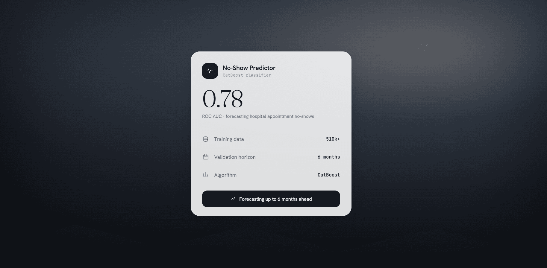
The final algorithm was CatBoost, not XGBoost, which served as the baseline during development. The practical difference between the two on this problem was marginal. What CatBoost handled more elegantly was native support for categorical variables without extensive manual encoding, which simplified the pipeline and reduced the risk of leakage from mishandling high-cardinality categories such as insurer and ICD code.
The choice of algorithm, however, was the least important decision in the project. That isn't modesty. It's what the data shows. The AUC difference between the main algorithms tested (CatBoost, XGBoost, Random Forest, and Logistic Regression as a baseline) was smaller than the difference produced by one well-built patient history feature.
What mattered more than the algorithm was the validation strategy.
Scheduling data has structural seasonality. If you split the dataset randomly into train and test, you inevitably use information from the future to train: a patient who missed an appointment in March shows up in training, and the same behavioral pattern sits in the January test set. The model learns to "remember" patterns that, in real production, would not have happened yet. The result is an inflated AUC that collapses when the model meets real prospective data.
The validation we adopted was temporal: train on history up to a defined cutoff, test on the following 6 months in chronological order. The model never saw future data during training. It is the only validation that mimics what would happen in production.
The resulting ROC-AUC was 0.78 on the temporal test. It is not the highest number this dataset can produce. With random validation, we reached higher values. It is, however, the number that represents the real performance to expect when the model is used prospectively.
The comparison with the global literature shows why that rigor matters.
Where this model stands in the global literature
Benchmarking against published studies was part of this project's scope, and the results are honest enough to report without cherry-picking.
We compared the model with no-show prediction studies in radiology and other specialties from major institutions: centers in the US (Massachusetts General Hospital, University of Maryland), Singapore (Changi General Hospital), Israel (Assuta Medical Centers), and Japan. Most published studies use random validation or less rigorous temporal cross-validation.
The pattern we found again and again: models that report an AUC of 0.90 or higher in testing, then drop to 0.73-0.74 when revalidated on real prospective data. One specific study published an AUC of 0.93 in cross-validation and 0.73 in prospective testing, a 20-point drop that only shows up when the methodology is honest about time.
Our model, trained and validated under the most restrictive protocol, delivers 0.78 on the prospective test. That puts it ahead of roughly 75% of comparable studies on real prospective performance, not on optimistic benchmark performance.
What makes the comparison valid: the dataset covers 15 or more different modalities in a single model (most studies are single-modality), and its volume of 510,000 records exceeds most published datasets in public healthcare settings.
What the pilot proposes, and what hasn't happened yet
The model exists. The validation exists. What doesn't exist yet is a system in production.
The pilot proposal, which is awaiting executive approval, is built around a smart overbooking mechanism that is fundamentally different from the blunt overbooking some institutions practice.
The logic is simple: the model generates a no-show probability score for each booking at the moment it is made. When that score crosses a threshold of roughly 70%, the system suggests to the scheduler that the slot can take an additional booking. The scheduler validates it. The suggestion is not automatic. It is statistically grounded decision support.
The proposed safety mechanisms matter as much as the suggestion itself:
- Overbooking cap per modality: a maximum of 10-15% additional slots per session, to prevent overcrowding if the model underestimates attendance
- Automatic stop rules: if actual overfill in any session exceeds 5%, or if wait time rises more than 30 minutes above the SLA, overbooking is automatically suspended for that day
- Hard clinical exceptions: patients with high-complexity exams or classified as urgent are 100% excluded from any overbooking logic, regardless of score
The philosophy guiding the design is "fail-safe": under any condition of uncertainty, the system reverts to default behavior. Zero harm to patients as a consequence of an incorrect model prediction.
The impact projections (recovery of 10-15% of current idle capacity, representing between R$1.5M and R$2.5M a year in additional capacity used) are estimates built on the model's performance and conservative assumptions about operational adoption. They are scenarios for a 90-day pilot, not observed results. The distance between a validated model and a production system is real, and closing that distance honestly is part of the project.
The model was designed as a replicable blueprint for other institutes within the same hospital complex, which face variations of the same problem with the same kind of data available.
How to replicate this architecture
If you are building a no-show prediction model for a hospital operation, these are the decisions that matter most, in order of real impact:
1. Define the target before you touch the data. A no-show is not the same as "didn't attend." Early cancellations, reschedules, and absences due to hospital admission each carry different semantics and deserve different treatment. Define the label the model needs to predict before building the dataset. An imprecise definition here contaminates everything that follows.
2. Spend most of your time on data engineering. The rule of thumb that emerged from this project: if you are spending less than 50% of the effort on cleaning, normalization, and source integration, you are probably underestimating the problem. Noisy features produce noisy models, regardless of the algorithm.
3. Use temporal validation, not random. If the data has seasonality (and hospital scheduling data does), random validation produces metrics that don't match prospective reality. Train on the past, test on the future. Accept any drop in AUC as information, not as failure.
4. Prioritize patient behavioral features. The patient's no-show history is consistently the strongest predictor in this domain. Before investing in sophisticated clinical features or elaborate temporal engineering, make sure patient history is well represented and clean in the dataset.
5. Do the descriptive analysis before the model. Temporal decomposition (SARIMAX or equivalent) and segmentation analyses reveal patterns that inform feature engineering and spare the model from having to "discover" what the data already shows plainly. Weekend slots from 8 p.m. to 10 p.m. with a 90% no-show rate are a schedule configuration problem, not a prediction problem.
6. Design the application mechanism with humans in charge. In systems that directly affect patient care, blind automation is the wrong risk to take. The model is a decision support tool: it informs the scheduler, it does not replace judgment. Build the override mechanisms, stop rules, and clinical exceptions before you think about deployment.
What we would do differently
Category normalization was done incrementally over the course of the project, fixing inconsistencies as they surfaced in the analysis. The right process would have been to build a canonical dictionary for each categorical variable (insurers, modalities, relevant ICD codes) before starting the cleanup. That would have saved multiple rounds of reprocessing the dataset.
Benchmarking against the literature was done fairly manually: reading papers, extracting metrics, comparing in a spreadsheet. For a project where comparison with published studies is part of the value argument, a more systematic benchmarking pipeline would have helped: a structured database of studies with standardized metrics, documented validation conditions, and automated comparison.
The analysis of error cost by type (false positive vs. false negative in the overbooking context) could have been formalized earlier. AUC is a useful discrimination metric, but the threshold decision for the overbooking suggestion depends on the operation's specific cost asymmetry: the cost of a wrongly suggested slot (the patient shows up, the room is full) versus the cost of an underused slot (a no-show nobody predicted). That analysis came late in the project.
The principle that connects this project to the data ecosystem
This no-show prediction project and the data agent we built for the same institution start from the same place (a vast, disorganized, and underused columnar data warehouse) and arrive at different destinations by different paths.
The data agent is reactive: a manager asks a question in natural language, and the agent translates it to SQL, runs it, interprets the result, and answers. The value lies in removing the human bottleneck between the question and the data.
This prediction model is proactive: without anyone asking, it analyzes every new booking and calculates the probability of a no-show. The value lies in acting before the event, not after.
Both projects turn the same disorganized data warehouse into operational value. The difference is temporal: one answers the present, the other anticipates the future. What unites them is the conviction that existing data, well worked, is worth more than any new data you could collect.
The data was already there. The work was understanding what it was saying, and building the layer that made it possible to listen to it systematically.
What is the difference between a no-show and a cancellation in this model?
The distinction is central to the model's usefulness. A no-show, as defined in this project, is a missed appointment without prior cancellation: the patient simply doesn't show up and never tells the institution. Cancellations, even last-minute ones, are separate records.
The reason for the separation is operational: a cancellation, even a late one, leaves some chance of reusing the slot. A no-show doesn't. The institution only finds out the patient missed the appointment when the time comes and the patient isn't there. That is the behavior that destroys capacity, and it is what the model was trained to anticipate.
Mixing the two labels in the target would produce a model that predicts "absence for any reason." That is useful for other purposes, but not for the smart overbooking mechanism this project proposes.
Why CatBoost and not XGBoost or another gradient boosting library?
XGBoost was the project's baseline and performed competitively. The choice of CatBoost as the final model was driven mainly by its native handling of categorical variables.
The dataset has high-cardinality features (insurer, ICD code, modality) that with XGBoost require explicit encoding (one-hot or target encoding). Target encoding under temporal validation needs extra care to avoid leakage. CatBoost handles categories directly, without external encoding, reducing pipeline complexity and the risk of implementation errors.
The AUC difference between the two was small, on the order of 0.01 to 0.02. The choice was about pipeline engineering, not raw performance.
Why does temporal validation matter more than standard cross-validation here?
Scheduling data has structural seasonality: no-show patterns vary by day of the week, month, time of year, and external events (holidays, public health campaigns, and so on). With random cross-validation, the model trains on December records and tests on January records, but it also trains on February records and tests on records from February of other years. Information "leaks" across time.
The practical result is an inflated AUC that doesn't match prospective performance. We publish 0.78 because that is the number obtained under the most restrictive protocol: train on the past, test on 6 chronologically later months the model never saw. It is the number that matters when deciding whether the model is useful in production.
The global literature shows this pattern again and again: models that report an AUC of 0.90+ with cross-validation drop to 0.73-0.74 when tested prospectively. Methodological honesty is part of the result.
Doesn't the overbooking mechanism risk harming patients?
That is the central design risk, and the pilot proposal was built to address it explicitly.
Three structural safeguards were designed. First, the suggestion threshold is conservative: only slots where the no-show probability score exceeds 70% receive an overbooking suggestion. That filters out most bookings. Second, the per-session cap limits overbooking to 10-15% of slots, so if the model underestimates attendance on a given day, the excess can be absorbed operationally. Third, automatic stop rules suspend overbooking if actual occupancy indicators exceed the defined thresholds.
On top of that, the suggestion is never automatic. The scheduler sees the score and decides. And patients with high-complexity or urgent exams are excluded regardless of score.
The principle governing the design is "fail-safe": under any condition of doubt, the system reverts to default behavior. The model can be wrong. The operational structure ensures the model's error doesn't turn into harm to the patient.
How is patient behavioral history calculated without violating privacy?
Behavioral history is calculated from the institution's own scheduling records, data it already holds and already uses operationally. It involves no external data collection, no cross-referencing with third-party databases, and no information beyond what is already in the scheduling system.
The features derived from that history are numerical aggregates: number of prior bookings, number of prior no-shows, historical attendance rate. No individual no-show record is exposed to the model as a feature, only aggregates that describe the patient's overall pattern.
The model processes this data inside the institution's internal environment. No patient information travels to external systems.